Model-Based Upstream Process Optimization
Introduction
What parameter values result in a desired outcome? – This is the question sought to be answered by systematically interrogated a process model with an optimization algorithm, deriving the set of parameter values that give rise to the desired performance. Imagine the possibilities when you can explore process regions that give rise to greater performance, efficiency, and excellence.
In this blog, we embark on exploring process optimization. From understanding the underlying principles to implementing practical strategies.
The objective
One of the questions during process development is typically that of process optimization, i.e. which combination of process parameter values (process condition), p , gives rise to a desired process outcome (such as maximum titer and/or adhering to a CQA fingerprint, etc). Hence, the objective of the process optimization is determined by what you aim to achieve.
For simplicity, let us assume you would want to maximize titer at the end of the process (Titer(tend)):

The enabler
For an algorithm to search which process condition, p, produces the desired process outcome, we need a model that links the process parameter values to the process outcome, i.e.:
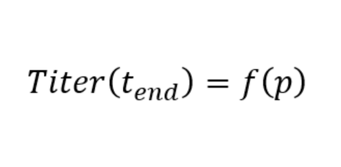
It is evident, that the more accurately the model describes the process behavior the better the outcome of the optimization exercise, i.e. how predictive is the model? Hybrid models which combine fundamental process knowledge with machine learning methods typically exhibit great predictivity, as they are able to describe the process behavior many times beyond what was tested experimentally, see e.g. here Understanding hybrid models in biochemical process systems.
The model might of course also capture the behavior of other process response variables (states), such as viable cell density, glucose, glutamine, lactate, ammonium, to name a few. In fact, a better understanding of the interplay of the response variables typically provides more process insight and subsequently, better results. So how can such a process model be obtained?
The start point
When starting process optimization, typically one encounters one of the following 3 scenarios:
Scenario 1 – Data from runs (experiments) are available for the product of interest:
In case you do have data from process runs available you can use them to create a first model. Using a generic hybrid modeling structure (see e.g. here), it is fairly straightforward to obtain a good performing model. While you might want to check the predictivity of your model (e.g. using a test set), using the model you can start the process optimization exercise. Note that the predictivity of the model will of course be constrained by the variation in the process parameters that was captured in the data, e.g. in case no temperature variations are covered in these run data, you might not expect the model to make predictions for various different temperatures. However, you can design variation into these variables for your next run, on top of using the models. Generally, we observe that the data that are available at this stage come from screening studies and hence have a good level of variation in almost all process parameters.
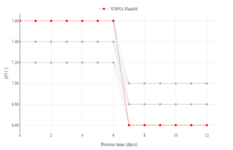 Figure 1: Different pH-profiles present in this campaign. One run is highlighted as an example.
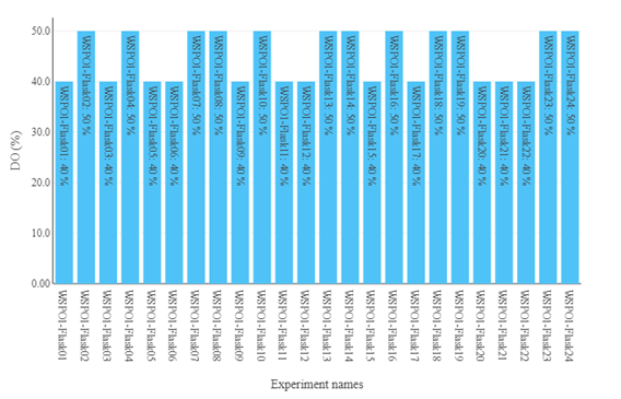 Figure 2: Different values of DO-set points present in this campaign.
For simplicity, let us assume that you (or a colleague) built a hybrid model, which describes the impact of the process parameters on the process response at every moment of time, as visualized in figure 3.
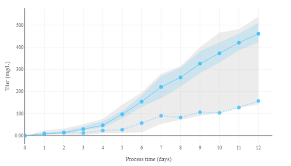 Figure 3: A hybrid model for the prediction of the process dynamics. By changing some parameters, the model now produces much higher titer. Blue dotted line: original data. Solid blue line: new prediction with updated parameters. Blue shaded area: confidence interval of prediction.
Scenario 2 – No data is available whatsoever:
The best option if no data is available, is to perform systematic variations in the process parameters, such that the model can learn how these variations impact on the process outcome. This is typically referred to as an excitation design (or engineering runs). It has been shown that for the application of machine-learning models, space-filling designs (such as Doehlert or Latin Hypercube Sampling) are particularly suitable. For instance, if you have four process parameters (temperature, pH, DO and stirring rate) and you can plan four process runs, the Latin Hypercube Sampling will provide you with the values of the four process parameters for the four runs. Table 1 shows an example of such an LHS design.
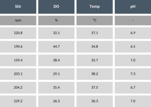 Table 1 – Example of process parameter values in LHS design.
We recommend performing at least as many runs as process parameters that you want to explore to obtain a good base for exploration. Besides the question of which process parameters to include in the optimization, the range of the process parameter values (bounds) which should be explored is important to be set carefully. On one hand, the range need to be large enough to see a difference in the process outcome (also considering the measurement error as well as run to run variation that you might have) and on the other hand, the range should be narrow enough to be able to explore the space (with a finite number of runs). Practically, for each process parameter you might use knowledge about past performance to set the bounds. Once you acquired the run data, continue with scenario 1.
Scenario 3 – Data from runs (experiments) are available for the same platform process but other products of interest:
In this blog, we will focus on scenarios 1 and 2, scenario 3 will be discussed in a later blog.
Getting the optimal conditions
Setting bounds: With a defined objective, a model in place, and awareness of its limitations, only the set-up of the optimization is missing. We choose the bounds for the process parameters that we want to explore and set the values for those that we want to keep fixed. In case we would like process parameters to vary over time, i.e. they are becoming functions rather than fixed parameters, we need to determine which function we would like to use to represent them.
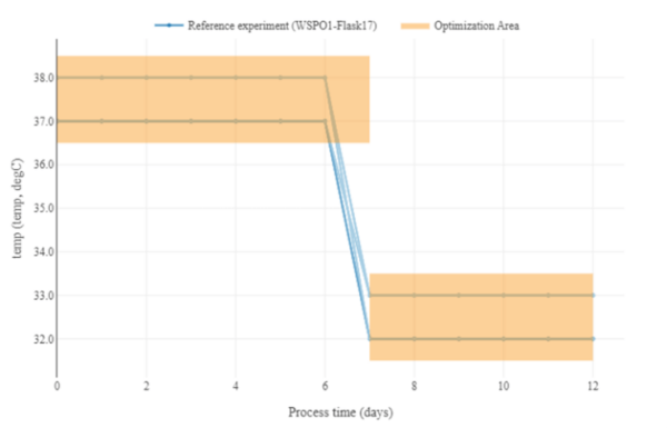 Figure 4: Ranges for the temperature profile, including a step to a lower temperature range on day 7.
For instance, we could choose a step-function for temperature, starting from 37°C until a certain time (here day 7) and then dropping to 33°C. Also, more complex functions like ramps, polynomials or exponentials (e.g. common for feeding profiles in the case of microbes) are possible, where the parameters of these functions become subject to the optimization.
Choosing optimization routine settings: The last point to consider is the number of iterations that you want the numerical optimization procedure to perform. The number of iterations is an expression for how long the optimization-algorithm is run. More iterations tend to explore the overall space better but cost more (computational) resources such as time. An (possibly local) optimal set of process parameters is found if the suggested values are not changing significantly anymore, between iterations. Examples of how experimental conditions that were found with an optimization could look like, are displayed in figure 5.
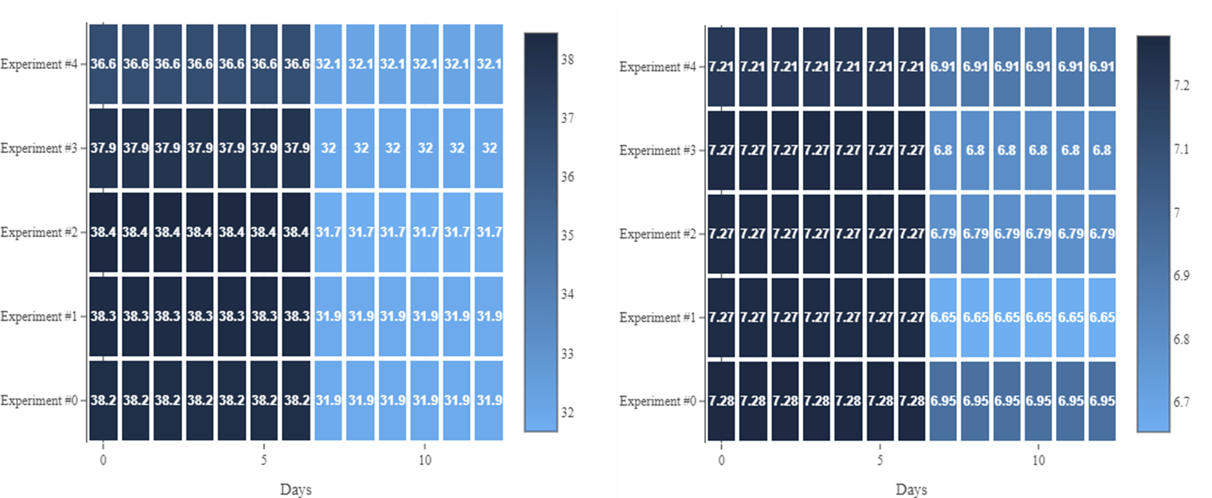 Figure 5: Examples of a design consisting of 5 experiments. The left-hand side shows temperature values, the right-hand side shows pH.
How sensible are these suggestions? This can be analyzed from two perspectives. The first is to check the model’s predictions for these conditions. Does the model predict an improvement in the objective function relative to the experiments already performed? On the other hand, how sure is the model of its predictions and are we entering unknown territory, meaning is the experimental condition associated with high risk of misspredicting?
The sanity check
The optimization routine is very effective in finding optimal conditions; however they might make sense only from a mathematical but not a process perspective. Hence, the suggested conditions should be evaluated and the temporal profiles visually inspected. In case the suggested optimal conditions are not sensible, you might modify the optimization settings and re-run the optimization routine. Alternatively, you could adapt the optimal solution slightly, making it feasible.
If you have multiple reactors available, there are strategies on how to make effective use of this capacity, for example by balancing exploitation and exploration. The former implies maximizing purely the quantity of interest, the latter aims to explore conditions where the model can learn the most while still in the vicinity of the optimum. For experimental settings, a great number of reactors (12+), we suggest to re-run at least one control condition from the original set of runs. This is done to assess the variation from campaign to campaign. Also, including replicates is beneficial to assess the process intrinsic variability.
The execution
Ready to implement the suggested optimal conditions? You might want to cross check the settings, as most runs fail at first due to oversight errors in the set-points. You could also consider having DataHowLAB communicating with your equipment directly, get in touch for more info.
The review
The good news is, you win every time. With the data from the new run(s) becoming available, you can use the model in combination with the data to assess whether there were major differences between planning and execution. This helps you to have a fairer assessment of the optimization performance. Here we typically experience two cases: 1. The prediction and experimental value match closely; 2. The prediction and experimental value differ considerately, and you obtained experimentally either more or less titer than previously.
In either case you win, as you might have either found the optimum or a great learning opportunity. While in the first case you might stop looking for better conditions, in the second case you might want to start all over. This is what is typically referred to as iterative optimization. However, you can have control over the likelihood of running into the second scenario using a risk of misprediction measure to constraint the optimization to regions where the model’s predictions are faithful, which we will describe in the next blog.